If you’ve ever needed to summarize thousands of rows of data in just a few clicks, PivotTables are your best friend. They allow you to group, filter, sort, and analyze information without needing complicated formulas.
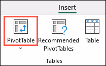
Start by selecting your dataset and choosing Insert → PivotTable. A new drag-and-drop panel appears where you can place fields into Rows, Columns, Values, and Filters. Instantly, your messy spreadsheet becomes a neatly summarized report—total sales by month, count of clients per region, average score by category, and more.
Formatting takes PivotTables to the next level. Apply PivotTable Styles for polished colors and borders, use Number Formatting for currency or percentages, and enable Subtotals and Grand Totals for clear breakdowns. You can also display the same data in different ways—sum, count, average, min/max—without rewriting anything.
Add PivotCharts and Slicers and you’ve built an interactive dashboard with minimal effort.
PivotTables save hours of manual sorting and calculation. If you’re working with large datasets, they are one of the most time-saving and powerful formatting tools Excel offers.
Learn more at Microsoft Support: https://support.microsoft.com/en-us/office/create-a-pivottable-to-analyze-worksheet-data-a9a84538-bfe9-40a9-a8e9-f99134456576